Self-experimentation in calibration

Set up

While taking two MITx courses on development policy: Foundations of Development Policy and The Challenges of Global Poverty, I had the opportunity to answer a great number of self-assessment questions.

For each of them, I noted down:

The question
The date
The type of question: {Multiple choice, Multiple selection, True or False, Enter a value}
Whether it was a question made during the lecture, given for homework, or part of an exam
My answer
Whether I got it right
Did I get it right the first time, or did I need a second try?
“My inner experience. One of {Hunch, Somewhat confident, Confident, Very confident, Incredibly Confident}
A short comment, if I felt like it.
My current mental state, according to the Becket Depression Checklist (only for the second half of the dataset; for the first part, the average value of the second part is given instead)
The probability I assign to my answer being correct, in odds form. For example, probabilities of 50%, 75%, 90% and 95% correspond to odds of 1:1, 1:3,1:9 and 1:19 respectively.

I have 505 observations. The dataset is available if I know you or if you can get someone who knows me to vouch for you.

1. How well calibrated am I?

A picture is worth a thousand words:

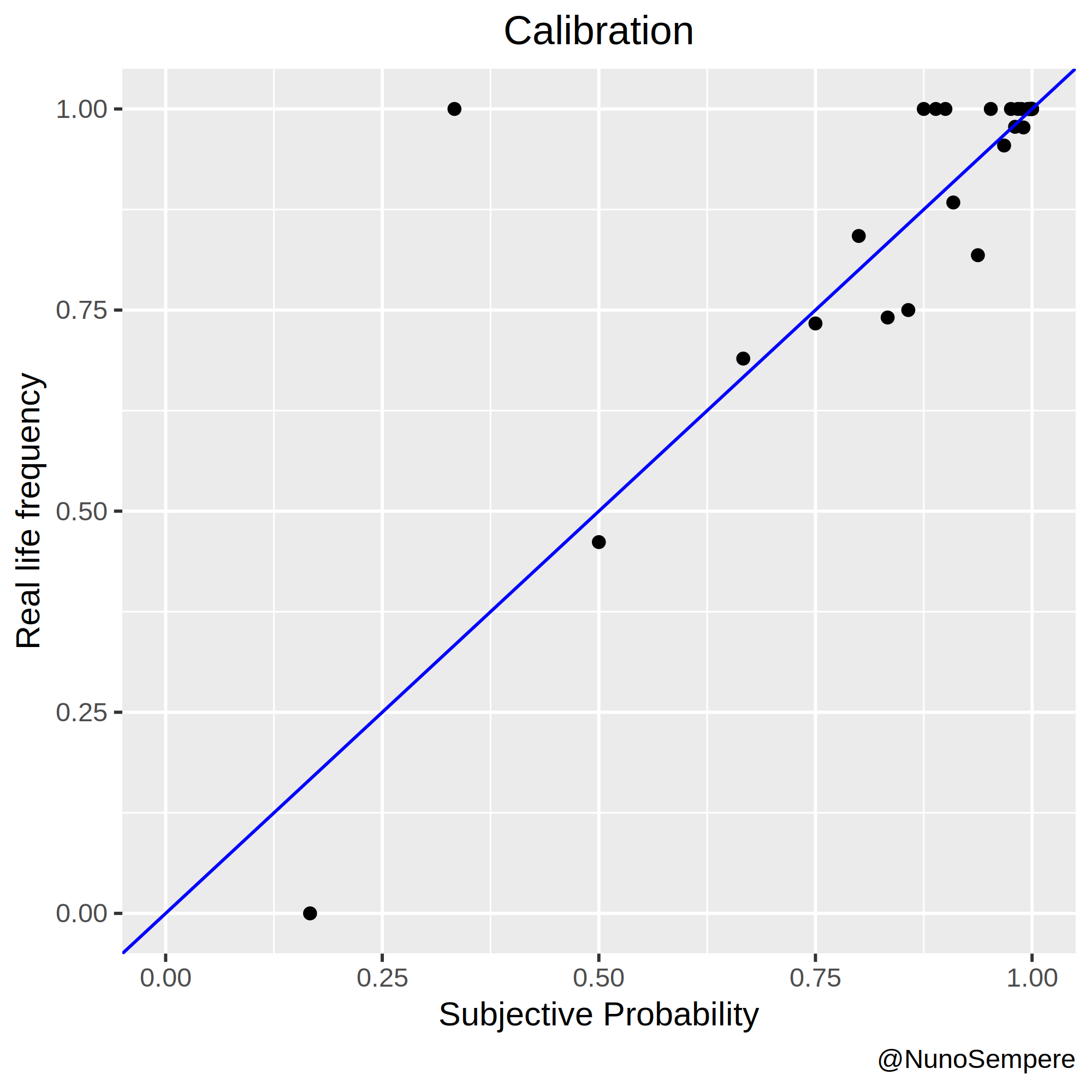
In this case, two pictures: The second merges probabilities > and < than .5 in the obvious way: it interprets having assigned a probability of, say, 0.33 to “X” as having assigned a probability of 0.66 to “Not X”. Working with odds, this is also straightforward: if you think that 1:2 are fair odds in favor of “X”, you also think that 2:1 are fair odds in favor of “Not X”.

I notice that my 1:5 is closer to 1:2.5 in reality, with n=28 observations. My 1:15 is also closer to 1:5, but I think that this particularity can be explained by 1:15 being the default value, i.e., the value which got written when I left that cell blank. I’ll nonetheless pay attention to that in the future. On the bright side, my 1:2 and 1:3 odds are exactly on point.

My Brier score is 0.0755985. The significant digits become relevant later.

2. How do I compare to a some simple regression models?

I created four simple linear regression models and interpret their output as probability. I also consider a really really dumb predictor, for comparison purposes.

The first one regresses the binary outcome (1 if true, 0 if false) on the variables 3,4,7 and 10 outlined in the set up. That is, I consider the type of question, whether it was homework, normal or part of an exam, my score in the BDC and whether it was the first try or not.
The second includes all the data outlined in the set up, except my subjective probability. Or, in other words, all the above + {Hunch, Somewhat confident, Confident, Very confident, Incredibly Confident} as factors.
The third only regresses binary outcome on my subjective probability.
The fourth includes all the numerical factors outlined in the setup.
The fifth model is really dumb, and just outputs as a probability my total base rate. There were 505 questions, I got 451 right, so it outputs a probability of 451/505 every time. If it only gets partial data, it calculates the base rate for the data it has, and always predicts that afterwards.

Here is a table:

	Which variable does the regression try to predict?	Variables regressed on (what information does this model work with)	Brier score tested & trained on the whole set	Trained on 80% and tested on the rest (average value, 1000+ times)	Trained on 50% and tested on the rest (average value, 1000+ times)
1. Dumbest model	Binary outcome	None. Empty regression, just the intercept	0.095496	0.09538288	0.09542671
2. Regression without any subjective factors	Binary outcome	1. Type of question 2. Homework vs Exam vs Lecture question 3. First vs second try 4. BDC	0.082598	0.131296	0.1412152
3. Regression model with inner experience	Binary outcome	1. Type of question 2. Homework vs Exam vs Lecture question 3. First vs second try 4. Becker Depression Checklist Score. 5. Inner experience: Hunch to Incredibly Confident	0.076962	0.1040722	0.1149272
4. Full regression model	Binary outcome	1. Type of question 2. Homework vs Exam vs Lecture question 3. First vs second try 4. Becker Depression Checklist Score. 5. Inner experience: Hunch to Incredibly Confident 6. Subjective probability	0.073224	0.09260587	0.1020023
5. Regression model with only my subjective probability	Binary outcome	1. Subjective probability	0.075541	0.07545493	0.07538371
6. Subjective probability	Does not apply	Not a regression model	Does not appy	Not a regression model	Does not apply	My Brier score was 0.0755985	-	-

2.1. Dumb model

A dumb model which always outputs the overall base rate gets a Brier score of 0.09549652. If I train it 1000 times on a randomly selected 80% of my data set and test it on the other 20% it still gets a 0.095-ish Brier score on average. By “train it”, I mean “regress the binary output on a constant variable of value 1”, or “calculate the base rate for that 80%, and use that”. It is surprising to me that this is does than some of the other models, some of the time.

2.2. Nothing subjective

2.2.1. Code and output

> summary(LM6)

Call:
lm(formula = Result_Binary ~ as.factor(D$Type.of.question) + Is_Normal + Is_Homework + BDC + as.factor(Trial..1st.if.not.specified.), 
    data = D)

Residuals:
     Min       1Q   Median       3Q      Max 
-1.00188  0.01493  0.04878  0.09309  0.49155 

Coefficients:
                                           Estimate Std. Error t value Pr(>|t|)   

(Intercept)                               0.8408927  0.0893759   9.408  < 2e-16 ***  
as.factor(D$Type.of.question)MC           0.1898829  0.0590873   3.214 0.001396 **  
as.factor(D$Type.of.question)MS          -0.0080026  0.0618861  -0.129 0.897163  
as.factor(D$Type.of.question)TF           0.1560246  0.0631872   2.469 0.013875 *  
Is_Normal                                 0.0342562  0.0453966   0.755 0.450848  
Is_Homework                              -0.0003015  0.0512829  -0.006 0.995311    
BDC                                      -0.0020370  0.0015640  -1.302 0.193366  
as.factor(Trial..1st.if.not.specified.)2 -0.2039517  0.0590451  -3.454 0.000599 ***  

Signif. codes:  0 ‘***’ 0.001 ‘**’ 0.01 ‘*’ 0.05 ‘.’ 0.1 ‘ ’ 1  

Residual standard error: 0.2897 on 497 degrees of freedom  
Multiple R-squared:  0.1349,	Adjusted R-squared:  0.1227  
F-statistic: 11.07 on 7 and 497 DF,  p-value: 4.899e-13  

2.2.2. Interpretation

I found it rather surprising that how depressed I was (BDC: Becker Depression Checklist) didn’t seem to have that big of an effect. In particular, I try to adjust for my mood, but I wasn’t particularly expecting to succeed. Anecdotically, I do see an effect of my mood on the extremity of my odds: The sadder I am the more recluctant I am to give 1:1000, 1:10000 and higher odds, even about things which I’m really sure about.

A multiple selection (MS) question can be thought of as a conjunction of several true or false (TF) questions, so the coefficient is lower. Surprisingly, though, multiple choice questions seem to be easier than true or false questions. This might be because for multiple choice questions the MITx team had a slight bias towards having the right answer be “a.”, which I detected and exploited. The other possible type of question is the one in which I’m asked to enter a value, which is unsurprisingly harder.

Otherwise, having needed a second try means that the question was hard, so there is accordingly a penalty. All in all, these coefficients seem reasonable.

If I use this model to output predicted probabilities for each question, I get a brier score of 0.0825985. If I instead train the model on a random selection of 80% of the data points, and test it on the other 20%, my answer depends on the specific selection. If I do that a 1000 times, I get a Brier score of 0.13-ish, on average. However, is this a result of having less data, or of having overfitted? To answer that, I trained the model on 50% of the data (selected randomly, 1000 times), and try to predict the other half, in which case it gets a Brier score of 0.14-ish, on average. Perhaps with more data it would have gotten to 0.12-ish, so the difference from that to 0.08-ish is probably a result of overfitting.

2.3. Everything except my subjective probablity

2.3.1. Code and output

> lm(Result_Binary ~ as.factor(D$Type.of.question) + as.factor(D$One.word) + Is_Normal + Is_Homework + BDC + as.factor(Trial..1st.if.not.specified.), data=D) -> LM1
> summary(LM1)

Call:
lm(formula = Result_Binary ~ as.factor(D$Type.of.question) + as.factor(D$One.word) + Is_Normal + Is_Homework + BDC + as.factor(Trial..1st.if.not.specified.), data = D)

Residuals:
     Min       1Q   Median       3Q      Max 
-1.00613 -0.00974  0.02935  0.10896  0.52292 

Coefficients:
                                          Estimate Std. Error t value Pr(>|t|)    
(Intercept)                               0.978323   0.165554   5.909 6.42e-09 ***
as.factor(D$Type.of.question)MC           0.118702   0.058962   2.013   0.0446 *  
as.factor(D$Type.of.question)MS           0.008630   0.060303   0.143   0.8863    
as.factor(D$Type.of.question)TF           0.079615   0.062979   1.264   0.2068    
as.factor(D$One.word)Confident           -0.093032   0.146151  -0.637   0.5247    
as.factor(D$One.word)Hunch               -0.273419   0.145842  -1.875   0.0614 .  
as.factor(D$One.word)IC                  -0.048987   0.143208  -0.342   0.7324    
as.factor(D$One.word)Somewhat confident  -0.113553   0.153972  -0.737   0.4612    
as.factor(D$One.word)Very confident      -0.063647   0.150520  -0.423   0.6726    
Is_Normal                                 0.042698   0.045620   0.936   0.3498    
Is_Homework                               0.018212   0.050816   0.358   0.7202    
BDC                                      -0.002064   0.001525  -1.353   0.1765    
as.factor(Trial..1st.if.not.specified.)2 -0.132914   0.059075  -2.250   0.0249 *  
---
Signif. codes:  0 ‘***’ 0.001 ‘**’ 0.01 ‘*’ 0.05 ‘.’ 0.1 ‘ ’ 1

Residual standard error: 0.2813 on 492 degrees of freedom
Multiple R-squared:  0.193,	Adjusted R-squared:  0.1733 
F-statistic: 9.804 on 12 and 492 DF,  p-value: < 2.2e-16

2.3.2 Interpretation

As expected, the coefficients associated with a measure of my inner confidence check out. Huch < Somewhat confident < Confident < Very confident < Incredibly confident (IC). Note that all of the factors are present, instead of one of them having been swallowed by the intercept, because there were 3 times which I just left that question blank, and I didn’t want to remove that data.

If I use this model to output predicted probabilities for each question, I get a brier score of 0.07696276. This is scarily close to my own Brier score of 0.0755985, until one realizes that a) The dataset in which this is tested is the same dataset in which the model has been trained, and b) it already contains some of my subjective information in the form of my inner experience.

If I instead train the model on a random selection of 80% of the data points, and test it on the other 20%, my answer depends on the specific selection. If I do that a 1000 times, I get a Brier score of 0.10-ish, on average. Again, the question arises of whether this is a result of having less data, or of having overfitted. To answer that, I again trained the model on 50% of the data (selected randomly, 1000 times), and try to predict the other half, in which case it gets a Brier score of 0.11-ish, on average. Perhaps with more data it would have gotten to 0.9-ish, so the difference from that to 0.07-ish is probably a result of overfitting.

2.4. Including my subjective probability & everything else.

2.4.1. Code and output

> summary(LM3)

Call:
lm(formula = Result_Binary ~ as.factor(D$Type.of.question) + 
    as.factor(D$One.word) + Is_Normal + Is_Homework + BDC + prob(D$for.) + 
    as.factor(Trial..1st.if.not.specified.), data = D)

Residuals:
     Min       1Q   Median       3Q      Max 
-1.00040 -0.01371  0.02636  0.10693  0.62249 

Coefficients:
                                          Estimate Std. Error t value Pr(>|t|)    
(Intercept)                               0.163526   0.230260   0.710   0.4779    
as.factor(D$Type.of.question)MC           0.096125   0.057770   1.664   0.0968 .  
as.factor(D$Type.of.question)MS           0.018922   0.058937   0.321   0.7483    
as.factor(D$Type.of.question)TF           0.054964   0.061714   0.891   0.3736    
as.factor(D$One.word)Confident           -0.024463   0.143417  -0.171   0.8646    
as.factor(D$One.word)Hunch               -0.031549   0.150532  -0.210   0.8341    
as.factor(D$One.word)IC                  -0.045438   0.139880  -0.325   0.7454    
as.factor(D$One.word)Somewhat confident  -0.045952   0.151005  -0.304   0.7610    
as.factor(D$One.word)Very confident      -0.040334   0.147095  -0.274   0.7840    
Is_Normal                                 0.039468   0.044564   0.886   0.3762    
Is_Homework                               0.029335   0.049685   0.590   0.5552    
BDC                                      -0.002599   0.001493  -1.740   0.0824 .  
prob(D$for.)                              0.867436   0.174515   4.971 9.24e-07 ***
as.factor(Trial..1st.if.not.specified.)2 -0.097659   0.058136  -1.680   0.0936 .  
---
Signif. codes:  0 ‘***’ 0.001 ‘**’ 0.01 ‘*’ 0.05 ‘.’ 0.1 ‘ ’ 1

Residual standard error: 0.2747 on 491 degrees of freedom
Multiple R-squared:  0.2316,	Adjusted R-squared:  0.2113 
F-statistic: 11.39 on 13 and 491 DF,  p-value: < 2.2e-16

2.4.1. Interpretation

All the other factors become slightly more irrelevant. It seems that my subjective probability does add information, a lot of it. After having seen the graph at the beginning, this is not surprising.

If I use this model to output probabilities for each question, I get a Brier score of 0.07322408, which is better than Brier score alone. As before, if I train this regression model on a random selection of 80% of the data points, and test it on the other 20%, my answer depends on the specific selection. If I do that a 1000 times and average the result, I get a Brier score of 0.9-ish. Again, the question arises of whether this is a result of having less data, or of having overfitted. To answer that, I again trained the model on 50% of the data (selected randomly, 1000 times), and try to predict the other half, in which case it gets a Brier score of 0.10-ish, on average. Perhaps with more data it would have gotten to 0.8-ish. To close a call.

2.5. Including only my subjective probability

2.5.1. Code and output

> summary(LM2)

Call:
lm(formula = Result_Binary ~ prob(D$for.), data = D)

Residuals:
     Min       1Q   Median       3Q      Max 
-0.98300  0.00906  0.01700  0.09842  0.67705 

Coefficients:
             Estimate Std. Error t value Pr(>|t|)    
(Intercept)  -0.01204    0.07947  -0.152     0.88    
prob(D$for.)  1.00499    0.08718  11.527   <2e-16 ***
---
Signif. codes:  0 ‘***’ 0.001 ‘**’ 0.01 ‘*’ 0.05 ‘.’ 0.1 ‘ ’ 1

Residual standard error: 0.2754 on 503 degrees of freedom
Multiple R-squared:  0.209,	Adjusted R-squared:  0.2074 
F-statistic: 132.9 on 1 and 503 DF,  p-value: < 2.2e-16

2.3.2. Interpretation

Multiply my probability by 1.005-ish and take 1.2% from that, and I’d be slightly more accurate. I’m not reading much into that. If I do this, I get an slightly better Brier score of 0.075541, slightly better than my own 0.0755985.

If, like before, I train that model 1000 times on a randomly selected 80% of my dataset, and test it on the other 20%, I get on average a Brier score of 0.07545493, slightly better than my own 0.0755985, but not by much. Perhaps it gets that slight advantage because the p*1.0005 - 1.2% corrects my uncalibrated 1:15 odds without murking the rest too much? Surprisingly, if I train it on a randomly selected 50% of the dataset (1000 times), its average Brier score improves to 0.07538371. I do not think that a difference of 0.002 tells me much.

3. Things I would do differently

If I were to redo this experiment, I’d:

Gather more data: I only used half the questions of the aforementioned course. 500 datapoints are really not that much.
Program a function to enter the data for me much earlier. Instead of doing that, I:
1. Started by writting my probabilities in my lecture notes, with the intention of cribbing them later. Never got around to doing that.
2. Started by writting it directly to a .csv myself
3. Saw that took too much time -> Wrote a couple of functions in R to do that for me
4. Saw that still took too much time -> Wrote a function to wrap the other functions. Everything went much more smoothly afterwards.
Use a scale other than the BDC: it’s not made for measuring daily moods.
Think through which data I want to collect from the beginning; I could have added the BDC from the start, but didn’t.

4. Conclusion

In conclusion, I am surprised that the dumb model beats the others most of the time, though I think this might be explained by the combination of not having that much data and of having a lot of variables: the random errors in my regression are large. I see that I am in general well calibrated (in the particular domain under analysis) but with room for improvement when giving 1:5, 1:6, and 1:15 odds.

Nuño Sempere

Measure is unceasing